Lecture: Data Manipulation and Transformation
Actuarial Data Science - Open Learning Resource
Recommended Reading
- R for Data Science, Chapters 3, 19
- Applied predictive Modelling, Chapters 3.3 (only transformations to resolve outliers), 3.4
Some coding examples in this lecture are adapted from R for Data Science (Wickham, Çetinkaya-Rundel, and Grolemund 2023).
Introduction
Motivation
- It is rare that you get the data in exactly the form you need.
- You may need to create new variables or summaries, or
- Simply rename variables or reorder observations to make the data easier to work with.
In practice, a large part of an actuary’s work involves cleaning and reshaping data to ensure that it is trustworthy and easy to analyse.
In this lecture, we introduce a small set of powerful verbs (filter(), select(), mutate(), summarise(), group_by(), and joins) that can be combined to express many common data-wrangling tasks clearly.
Using R to Manipulate Data
- R package:
dplyr(a core member oftidyverse) for data manipulation and transformation- Note:
dplyroverwrites some functions in base R (e.g.filter(),lag()). To use the base versions (after loadingdplyr), specifystats::filter()andstats::lag().
- Note:
- Data: the
nycflights13package, which contains data on flights departing from New York City in 2013 - We use
ggplot2to help us explore and understand the data.
Data
Types of variables
int: integersdbl: doubles (real numbers)chr: character vectors (strings)dttm: date-times (a date + time)lgl: logical vectors (TRUE or FALSE)fctr: factors (categorical variables with fixed levels)date: dates.
These are the common variable types used in tidyverse data frames (tibble)
Data Manipulation Functions
Functions for Data Manipulation
Functions in the dplyr package:
%>%: pipe operator, used to chain multiple operations togetherglimpse(): a glimpse into the data and its structurefilter(): select observations (rows) that satisfy given conditionsarrange(): reorder rows based on variable values
select(): choose a subset of variables (columns)mutate(): create new variables or transform existing onessummarise(): reduce multiple values to a single summarygroup_by(): group data so operations are performed within each group
Filter: Introduction
Filter: Comparisons
To use filter() effectively, you need to know how to select observations using comparison operators. R provides the standard set:
>greater than
>=greater than or equal to<less than
<=less than or equal to!=not equal to==equal to
Note: be cautious when using == with floating point numbers. Consider using near() instead.
Filter: Logical Operators
- Multiple arguments in
filter()are combined with “and”: every condition must be true for a row to be included in the output.
Other logical operators:
&: “and”|: “or”!: “not”x %in% yselect rows wherexis one of the values iny
According to De Morgan’s laws:
!(x & y)is equivalent to!x | !y!(x | y)is equivalent to!x & !y
Exercise: Filtering Multiple Months
Question:
Find all flights that departed in November or December.
Exercise: Combining Logical Conditions
Question:
Find flights that were not delayed (on arrival or departure) by more than two hours.
Filter: Missing Values
NArepresents an unknown value, so missing values are “contagious”: almost any operation involving an unknown value will also returnNA.filter()only includes rows where the condition isTRUE; it excludes bothFALSEandNAvalues. If you want to preserve missing values, you need to include them explicitly:
Arrange
arrange(): order rows by column names (or more complex expressions)- Use
desc()to sort a column in descending order - Missing values are always placed at the end
Select
select(): select a subset of variables (columns) by name
Select: Useful Functions
starts_with("abc"): select variables whose names begin with “abc”ends_with("xyz"): select variables whose names end with “xyz”contains("ijk"): select variables whose names contain “ijk”.matches(): select variables that match a regular expression.everything(): select all variables
Other related functions:
rename(): rename variablesmutate(): create new variables from existing variables
Summarise
Summarise with Group-by
- This changes the unit of analysis from the entire dataset to individual groups.
Exercise: Summarising Flight Delays by Destination
- Explore the relationship between distance and average delay for each destination
- There are three steps to prepare this data:
- Group flights by destination
- Summarise to compute distance, average delay, and number of flights
- Filter to remove noisy points (counts less than or equal to 20) and Honolulu (“HNL”) airport, which is much farther away than other destinations
Please have a try!
Solution: Data Manipulation
# Step 1: Group flights by destination
by_dest <- group_by(flights, dest)
# Step 2: Summarise to compute statistics for each destination
delay_summary <- summarise(by_dest,
count = n(), # Number of flights
dist = mean(distance, na.rm = TRUE), # Average distance
delay = mean(arr_delay, na.rm = TRUE) # Average arrival delay
)
# Step 3: Filter to remove noisy points and outliers
delay_summary <- filter(delay_summary,
count > 20, # Keep destinations with >20 flights
dest != "HNL") # Remove Honolulu (outlier: very far)
# Create visualization: relationship between distance and delay
# It looks like delays increase with distance up to ~750 miles
# and then decrease. Maybe as flights get longer there's more
# ability to make up delays in the air?
delay_plot <- ggplot(data = delay_summary,
mapping = aes(x = dist, y = delay)) +
geom_point(aes(size = count), alpha = 1/3) + # Point size represents flight count
geom_smooth(se = FALSE) # Add smooth trend line
#> `geom_smooth()` using method = 'loess' and formula 'y ~ x'Solution: Visualisation

Alternative Solution Using the Pipe Operator %>%
# Same analysis using pipe operator for cleaner, more readable code
delays_summary <- flights %>%
group_by(dest) %>% # Group by destination
summarise(
count = n(), # Number of flights per destination
dist = mean(distance, na.rm = TRUE), # Average distance
delay = mean(arr_delay, na.rm = TRUE) # Average arrival delay
) %>%
filter(count > 20, dest != "HNL") # Filter: >20 flights, exclude HonoluluMissing values
na.rm=TRUE: removes missing values
Useful Summary Functions
- Measures of location (central tendency):
mean(x),median(x) - Measures of spread (variability):
sd(x),IQR(x) - Measures of rank:
min(x),quantile(x, 0.25),max(x) - Measures of position:
first(x),nth(x, 2),last(x) - Counts:
n(),sum(!is.na(x)),n_distinct(x)count(tailnum, wt = distance): “count” (sum) the total number of miles a plane flew
- Counts and proportions of logical values:
sum(x > 10),mean(y == 0)
Note:
The interquartile range (IQR) is a measure of variability based on dividing a data set into quartiles. Q1 is the middle value in the lower half of the rank-ordered data. Q2 is the median value in the dataset. Q3 is the middle value in the upper half of the rank-ordered data. The interquartile range is equal to Q3 − Q1.
Grouping by Multiple Variables
Ungrouping
Relational Data
Relational Data
- Relational data: data stored across multiple tables that are related to each other
Three families of verbs designed to work with relational data:
Mutating joins: add new variables to one data frame from matching observations in another
Filtering joins: filter observations from one data frame based on whether they match observations in another table
Set operations: treat observations as if they were set elements.
A similar database system: SQL
Dataset
nycflights13contains five related tibbles:flights: information about each flightairlines: full carrier namesairports: information about each airport, identified by thefaaairport codeplanes: information about each plane, identified by itstailnumweather: weather data at each NYC airport for each hour
Table Relationships
- Each relationship involves a pair of tables
- It is important to understand how tables are connected when working with relational data
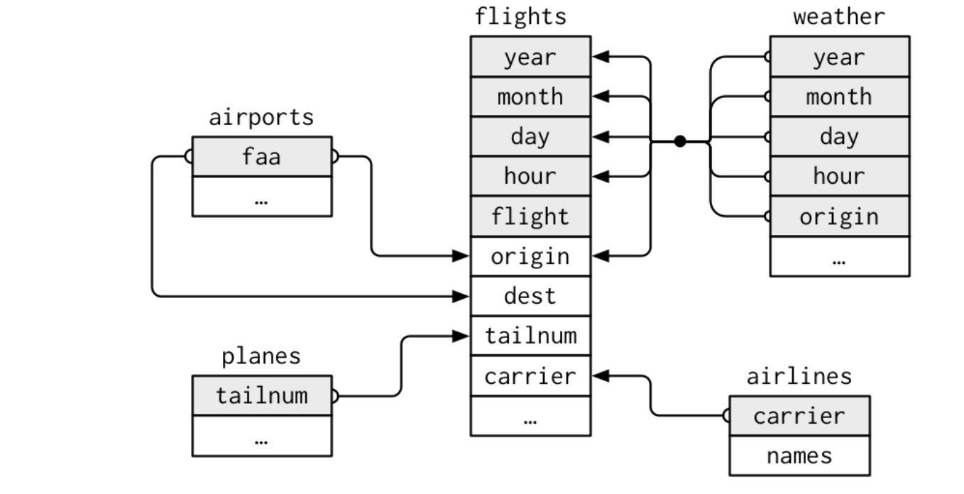
Relations of Tibbles (Source: Wickham and Grolemund (2017), R for Data Science)
Keys
- Primary key: a variable (or set of variables) that uniquely identifies each observation in its own table.
- For example,
planes$tailnumis a primary key because it uniquely identifies each plane in theplanestable.
- For example,
- Foreign key: a variable (or set of variables) in one table that refers to a primary key in another table.
- For example,
flights$tailnumis a foreign key because it links each flight to a plane in theplanestable.
- For example,
- A variable can be both a primary key and a foreign key. - For example,
originis part of the primary key in theweathertable, and is also a foreign key that links to theairportstable.
Identify the primary keys
- Use
count()the primary keys and look for entries wherenis greater than 1.
Add a Primary Key
- What is the primary key in the
flightstable?- None
- Surrogate key: add a primary key using
mutate()androw_number() - A primary key and the corresponding foreign key in another table form a relationship.
- Relationship are typically one-to-many. Many-to-many relationships can be represented using a many-to-one relationship plus a one-to-many relationship.
Exercise: Add a Surrogate Key to flights
flights %>%
arrange(year, month, day, sched_dep_time, carrier, flight) %>%
mutate(flight_id = row_number()) %>%
#This makes it possible to see every column in a data frame.
glimpse()Rows: 336,776
Columns: 20
$ year <int> 2013, 2013, 2013, 2013, 2013, 2013, 2013, 2013, 2013, 2~
$ month <int> 1, 1, 1, 1, 1, 1, 1, 1, 1, 1, 1, 1, 1, 1, 1, 1, 1, 1, 1~
$ day <int> 1, 1, 1, 1, 1, 1, 1, 1, 1, 1, 1, 1, 1, 1, 1, 1, 1, 1, 1~
$ dep_time <int> 517, 533, 542, 544, 554, 559, 558, 559, 558, 558, 557, ~
$ sched_dep_time <int> 515, 529, 540, 545, 558, 559, 600, 600, 600, 600, 600, ~
$ dep_delay <dbl> 2, 4, 2, -1, -4, 0, -2, -1, -2, -2, -3, NA, 1, 0, -5, -~
$ arr_time <int> 830, 850, 923, 1004, 740, 702, 753, 941, 849, 853, 838,~
$ sched_arr_time <int> 819, 830, 850, 1022, 728, 706, 745, 910, 851, 856, 846,~
$ arr_delay <dbl> 11, 20, 33, -18, 12, -4, 8, 31, -2, -3, -8, NA, -6, -7,~
$ carrier <chr> "UA", "UA", "AA", "B6", "UA", "B6", "AA", "AA", "B6", "~
$ flight <int> 1545, 1714, 1141, 725, 1696, 1806, 301, 707, 49, 71, 79~
$ tailnum <chr> "N14228", "N24211", "N619AA", "N804JB", "N39463", "N708~
$ origin <chr> "EWR", "LGA", "JFK", "JFK", "EWR", "JFK", "LGA", "LGA",~
$ dest <chr> "IAH", "IAH", "MIA", "BQN", "ORD", "BOS", "ORD", "DFW",~
$ air_time <dbl> 227, 227, 160, 183, 150, 44, 138, 257, 149, 158, 140, N~
$ distance <dbl> 1400, 1416, 1089, 1576, 719, 187, 733, 1389, 1028, 1005~
$ hour <dbl> 5, 5, 5, 5, 5, 5, 6, 6, 6, 6, 6, 6, 6, 6, 6, 6, 6, 6, 6~
$ minute <dbl> 15, 29, 40, 45, 58, 59, 0, 0, 0, 0, 0, 0, 0, 0, 0, 0, 0~
$ time_hour <dttm> 2013-01-01 05:00:00, 2013-01-01 05:00:00, 2013-01-01 0~
$ flight_id <int> 1, 2, 3, 4, 5, 6, 7, 8, 9, 10, 11, 12, 13, 14, 15, 16, ~Mutating Joins
- Mutating join combine variables from two tables. They match observations by their keys, then add variable from one table to the other.
- Add columns from
ytox:inner_join(): keep observations that appear in both tablesleft_join(): keep all observations inxright_join(): keep all observations inyfull_join(): keep all observations in bothxandy
Mutating Joins: Key Columns
- If keys are duplicated, the join returns all possible combinations of matching rows.
- Defining key columns
by=NULL: uses all variables that appear in both tables (a natural join)by = "x": uses a common variable named “x”by = c("a" = "b"): match variableain tablexto variablebin tabley
Mutating Joins: base::merge()
| dplyr | merge |
|---|---|
inner_join(x, y) |
merge(x, y) |
left_join(x, y) |
merge(x, y, all.x = TRUE) |
right_join(x, y) |
merge(x, y, all.y = TRUE) |
full_join(x, y) |
merge(x, y, all.x = TRUE, all.y = TRUE) |
dplyrjoins are generally faster and preserve the order of rows.
Filtering Joins
- Filtering joins match observations in the same way as mutating joins, but they affect rows (observations), not columns (variables).
- There are two types:
semi_join(x, y): keep all observations inxthat have a match inyanti_join(x, y): drop all observations inxthat have a match iny
Exercise: Using semi_join()
Question:
- Find the ten most popular destinations
- Match them back to
flights
# Step 1: Find top 10 most popular destinations
top_dest <- flights %>%
count(dest, sort = TRUE) %>% # Count flights per destination, sort descending
head(10) # Keep only top 10
# Step 2: Filter flights to only those going to top destinations
flights %>%
semi_join(top_dest) # Keep only flights matching top destinationsExercise: Using anti_join()
Question:
When connecting flights and planes, which flights do not have a match in in planes?
Join Problems
- Start by identifying the variables that form the primary key in each table.
- Check that none of the variables in the primary key are missing. If a value is missing, it cannot identify an observation.
- Check that your foreign keys match primary keys in another table. The best way to do this is using
anti_join().
Set Operations
intersect(x, y): return observations that appear in bothxandyunion(x, y): return all unique observations inxandysetdiff(x, y): return observations inxbut not iny
Examples of Set Operations
References