Lecture: Modelling and Shrinkage techniques
Actuarial Data Science - Open Learning Resource
Modelling Example: Polynomial Curve Fitting
- We simulate artificial training data from the function \sin(2\pi x) + \text{Gaussian random noise}, \quad x \in [0,1]
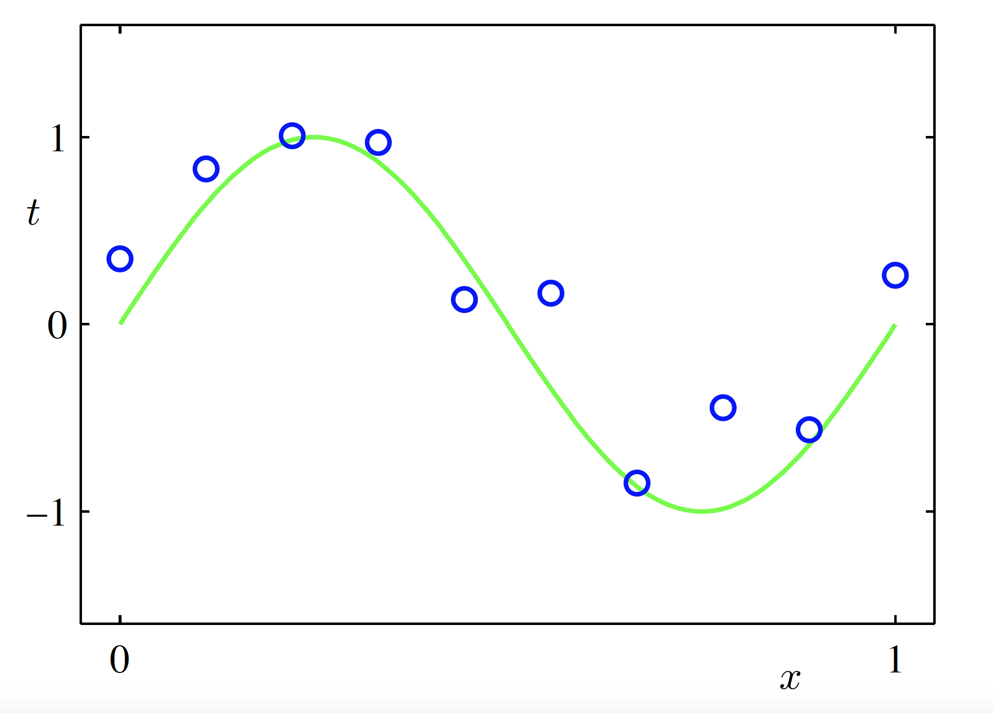
Data generation (Source: Bishop and Nasrabadi (2006), Figure 1.2)
Performance Measure
- Minimise an error function, such as the sum of squared errors \mathrm{Err}(\bm{w}) = \sum_{n=1}^{N} \bigl(f(x_n, \bm{w}) - y_n\bigr)^2
- A unique closed-form solution \bm{w}^* that minimises \mathrm{Err}(\bm{w}) can be obtained
- How should we choose the order M of the polynomial?
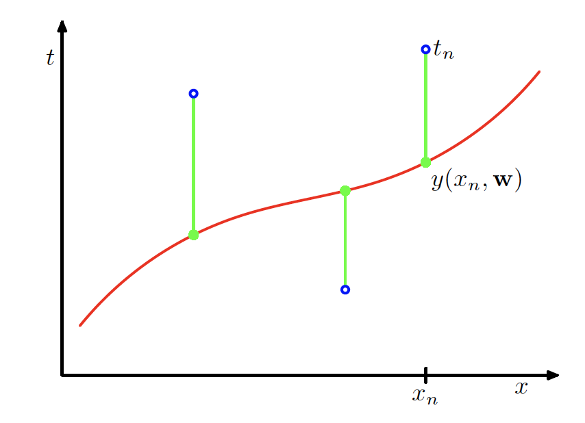
Geometric interpretation of the sum-of-squares error function (Source: Bishop and Nasrabadi (2006), Figure 1.3)
Constant Model (M = 0)
\begin{aligned} f(x, \bm{w}) &= \sum_{m=0}^{M} w_m x^m \Big|_{M=0} \\ &= w_0 \end{aligned}
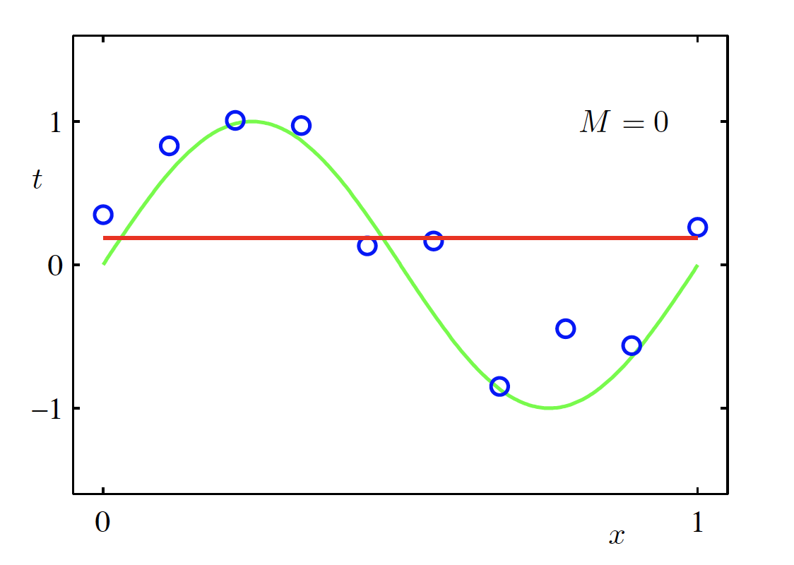
Fitted polynomial (M = 0) (Source: Bishop and Nasrabadi (2006), Figure 1.4)
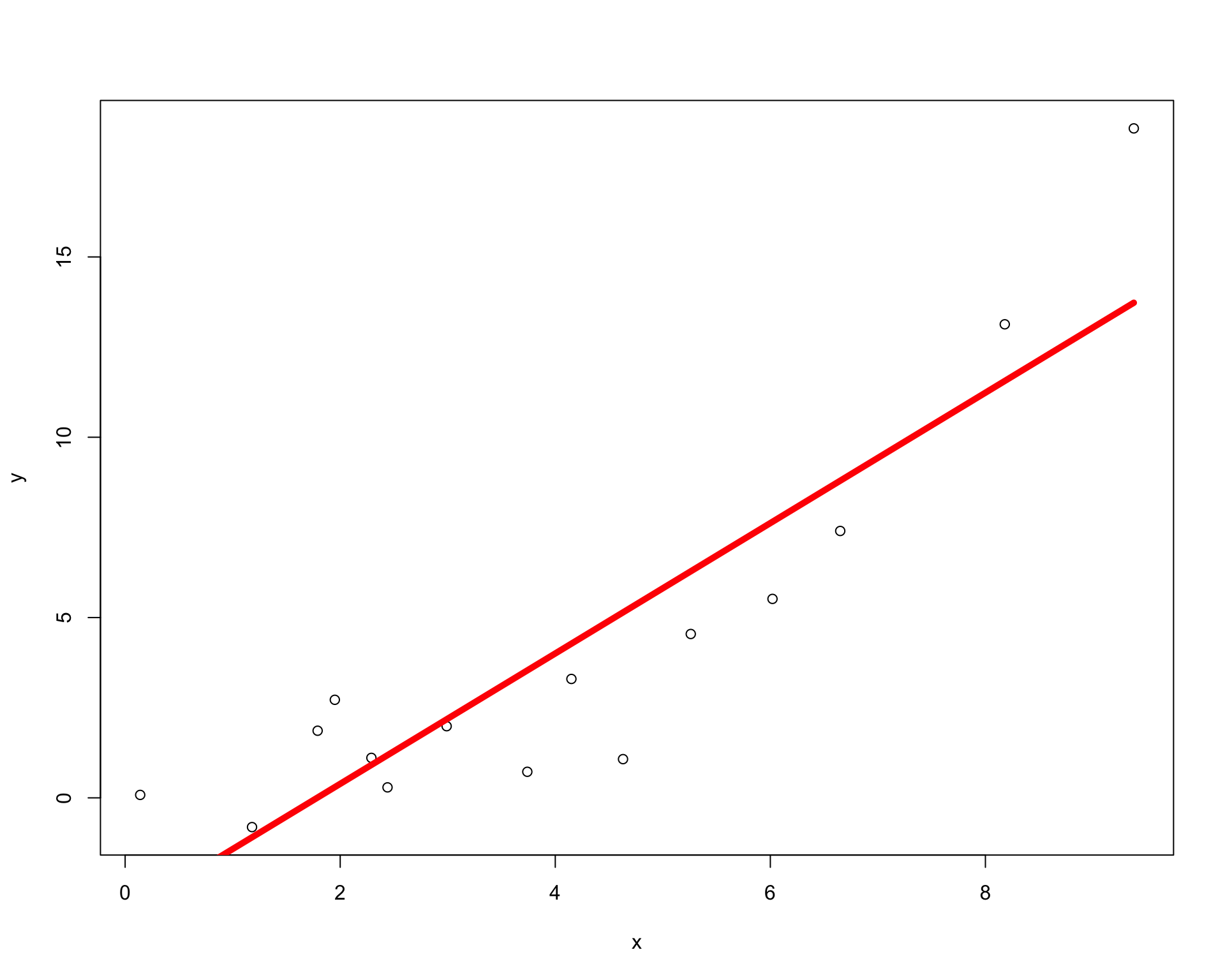
Linear Model (M = 1)
\begin{aligned} f(x, \bm{w}) &= \sum_{m=0}^{M} w_m x^m \Big|_{M=1} \\ &= w_0 + w_1 x \end{aligned}
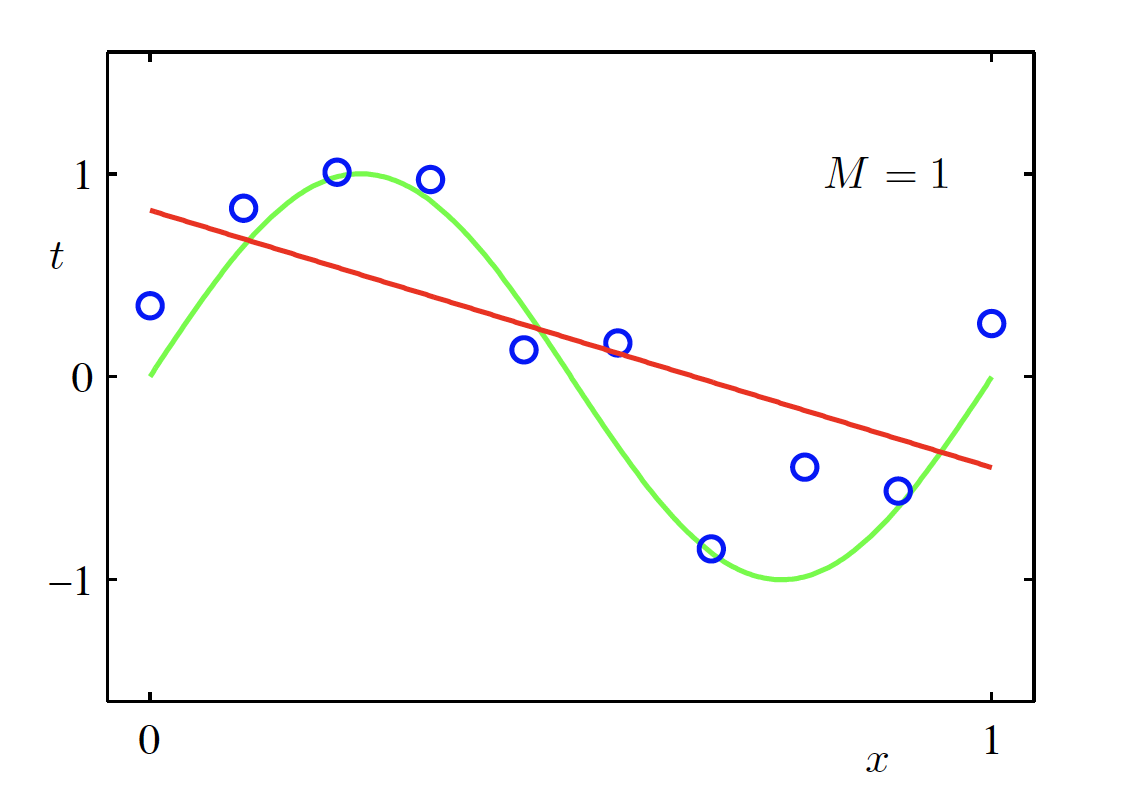
Fitted polynomial (M = 1) (Source: Bishop and Nasrabadi (2006), Figure 1.4)
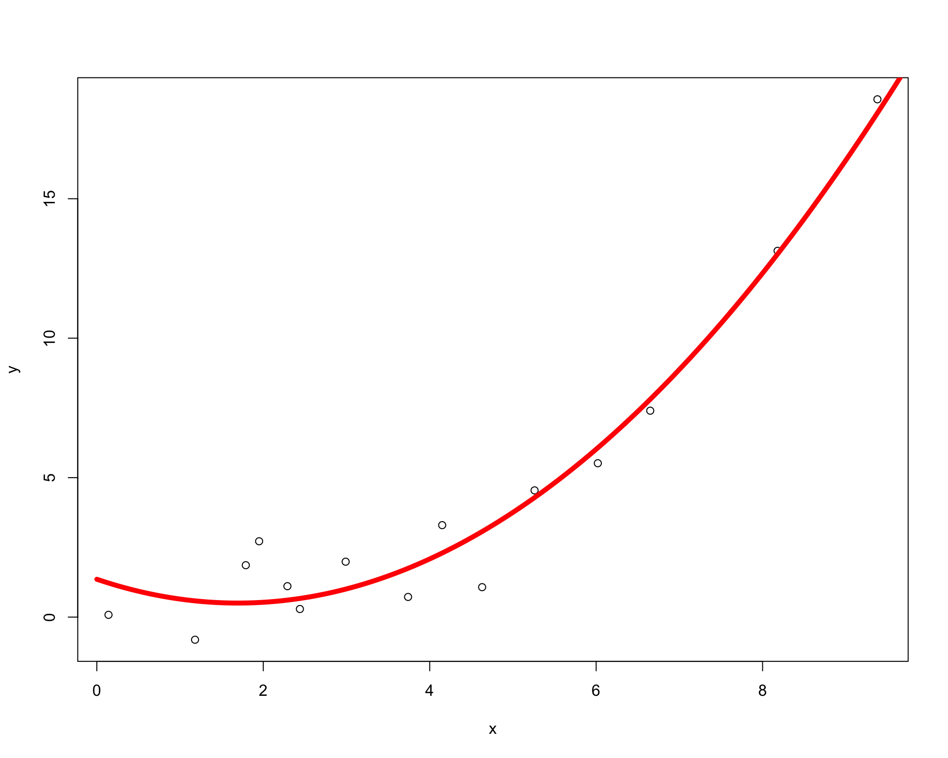
Cubic Polynomial Model (M = 3)
\begin{aligned} f(x, \bm{w}) &= \sum_{m=0}^{M} w_m x^m \Big|_{M=3} \\ &= w_0 + w_1 x + w_2 x^2 + w_3 x^3 \end{aligned}
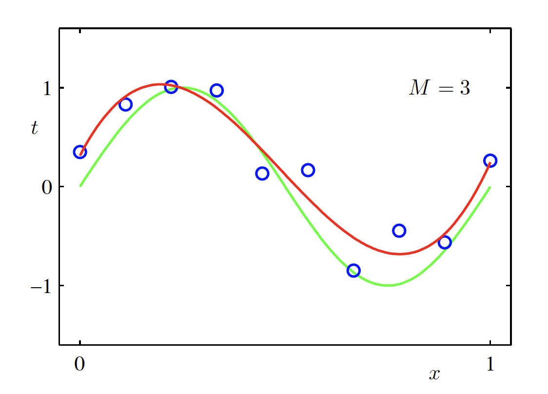
Fitted polynomial (M = 3) (Source: Bishop and Nasrabadi (2006), Figure 1.4)
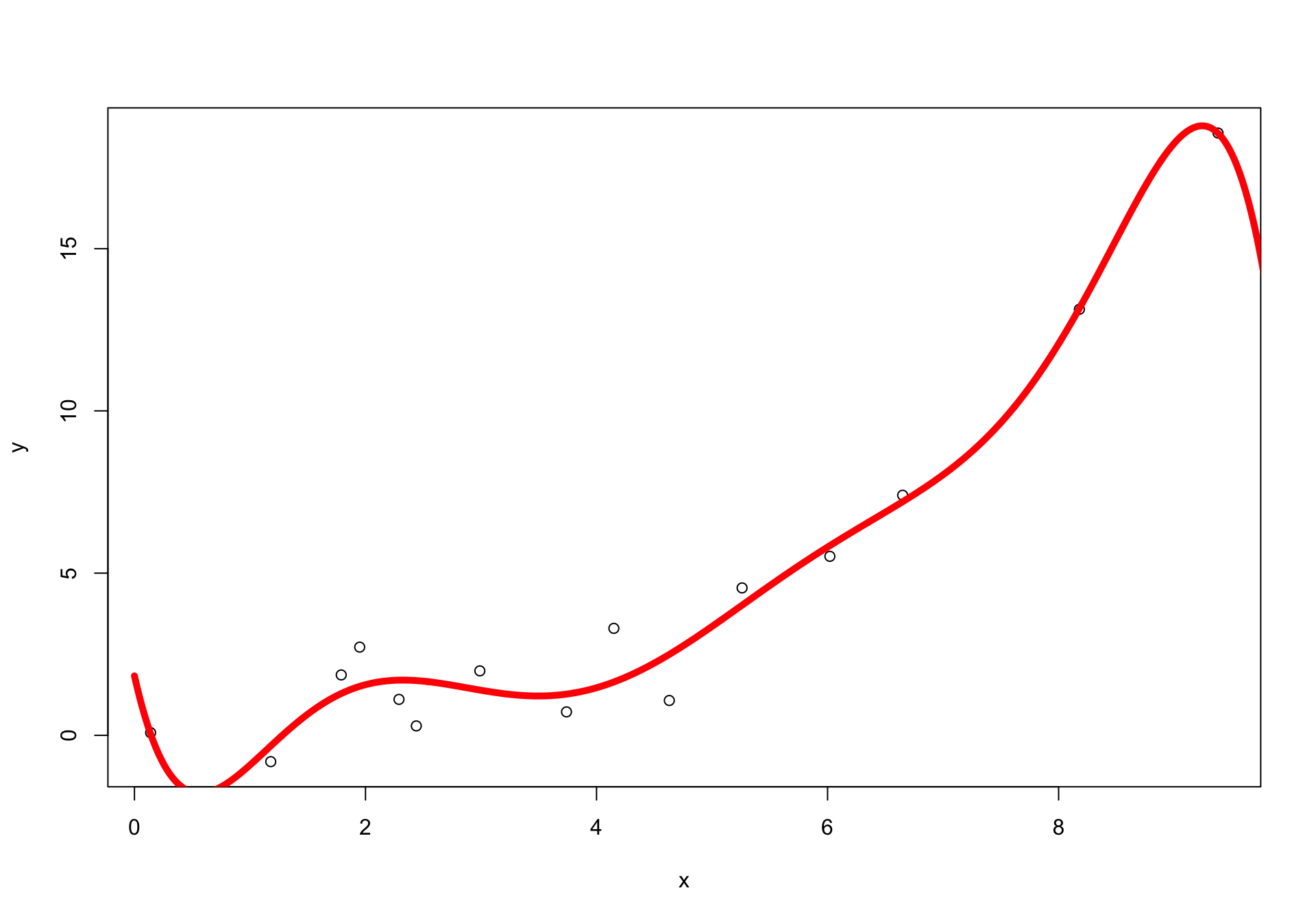
High-Degree Polynomial Model (M = 9)
\begin{aligned} f(x, \bm{w}) &= \sum_{m=0}^{M} w_m x^m \Big|_{M=9} \\ &= w_0 + w_1 x + \cdots + w_9 x^9 \end{aligned}
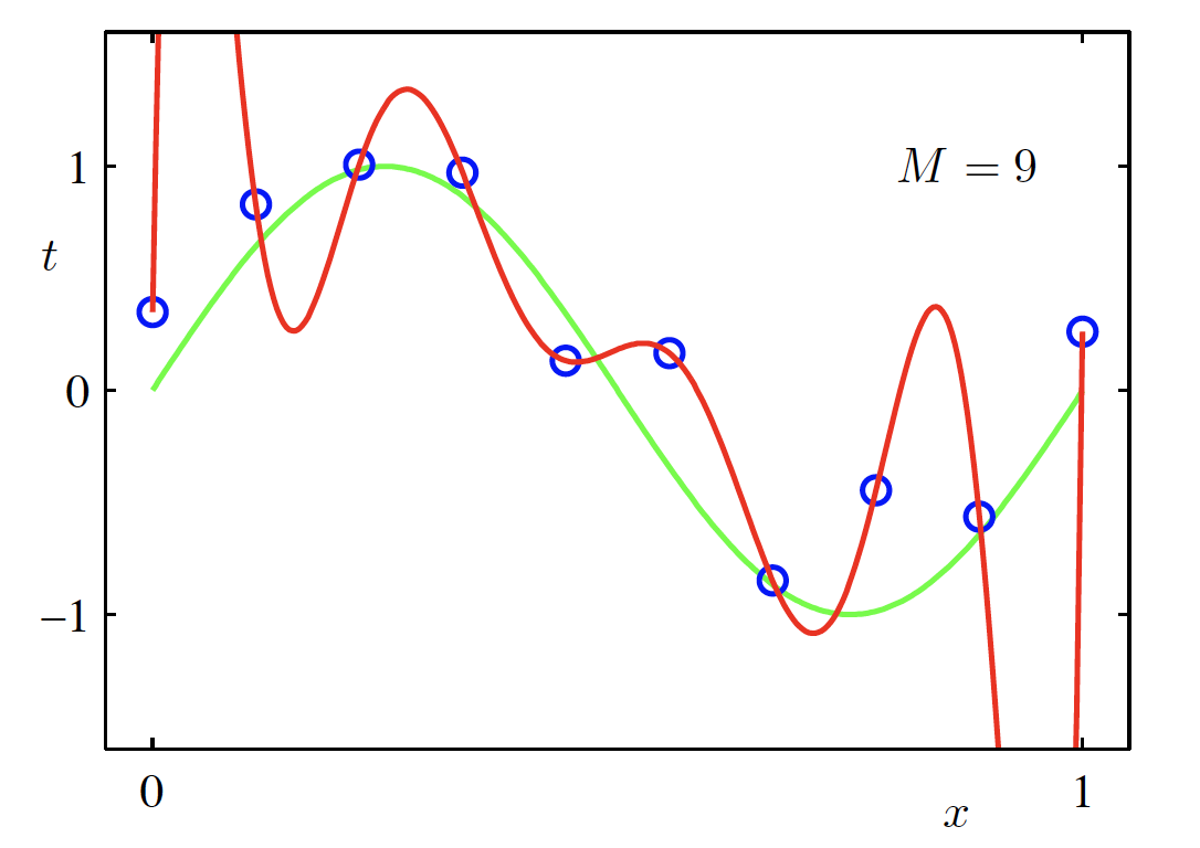
Fitted polynomial (M = 9) (Source: Bishop and Nasrabadi (2006), Figure 1.4)
Testing the Fitted Model
- Train the model and obtain \bm w^*
- Generate 100 new observations as a test set
- Root-mean-square (RMS) error Err_{RMS}=\sqrt{2Err(\bm w^*)/N}
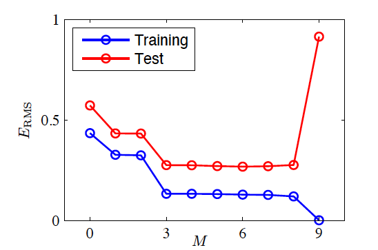
Training and test error vs model complexity (Source: Bishop and Nasrabadi (2006), Figure 1.5)
Parameters of the Fitted Model
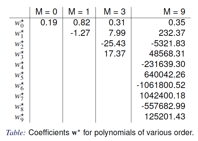
Fitted model parameters for different polynomial orders (Source: Bishop and Nasrabadi (2006), Table 1.1)
Effect of Training Data Size
- N=15, M=9
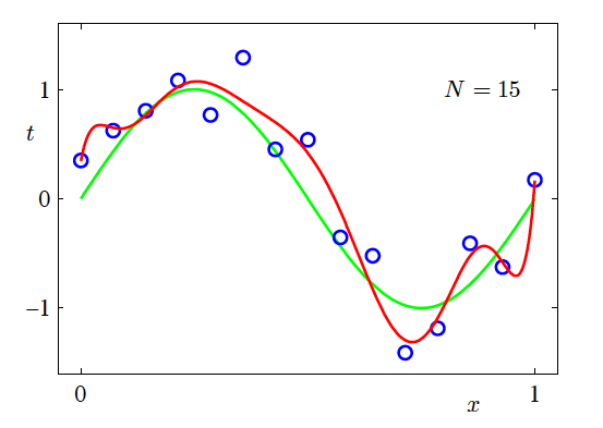
Effect of training set size on model fitting (N = 15, M = 9) (Source: Bishop and Nasrabadi (2006), Figure 1.6)
Increasing the Training Data Size
- N=100, M=9
- Increasing the size of the dataset reduces overfitting
- The number of data points should be no less than some multiple (say 5 or 10) of the number of parameters in the model
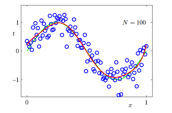
Effect of training set size on model fitting (N = 100, M = 9) (Source: Bishop and Nasrabadi (2006), Figure 1.6)
Data Spliting and Cross Validation
- Split the data into training, validation and testing sets
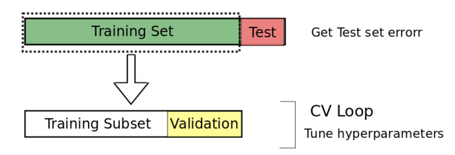
Data splitting (Source: Cochrane (2018))
- Cross validation
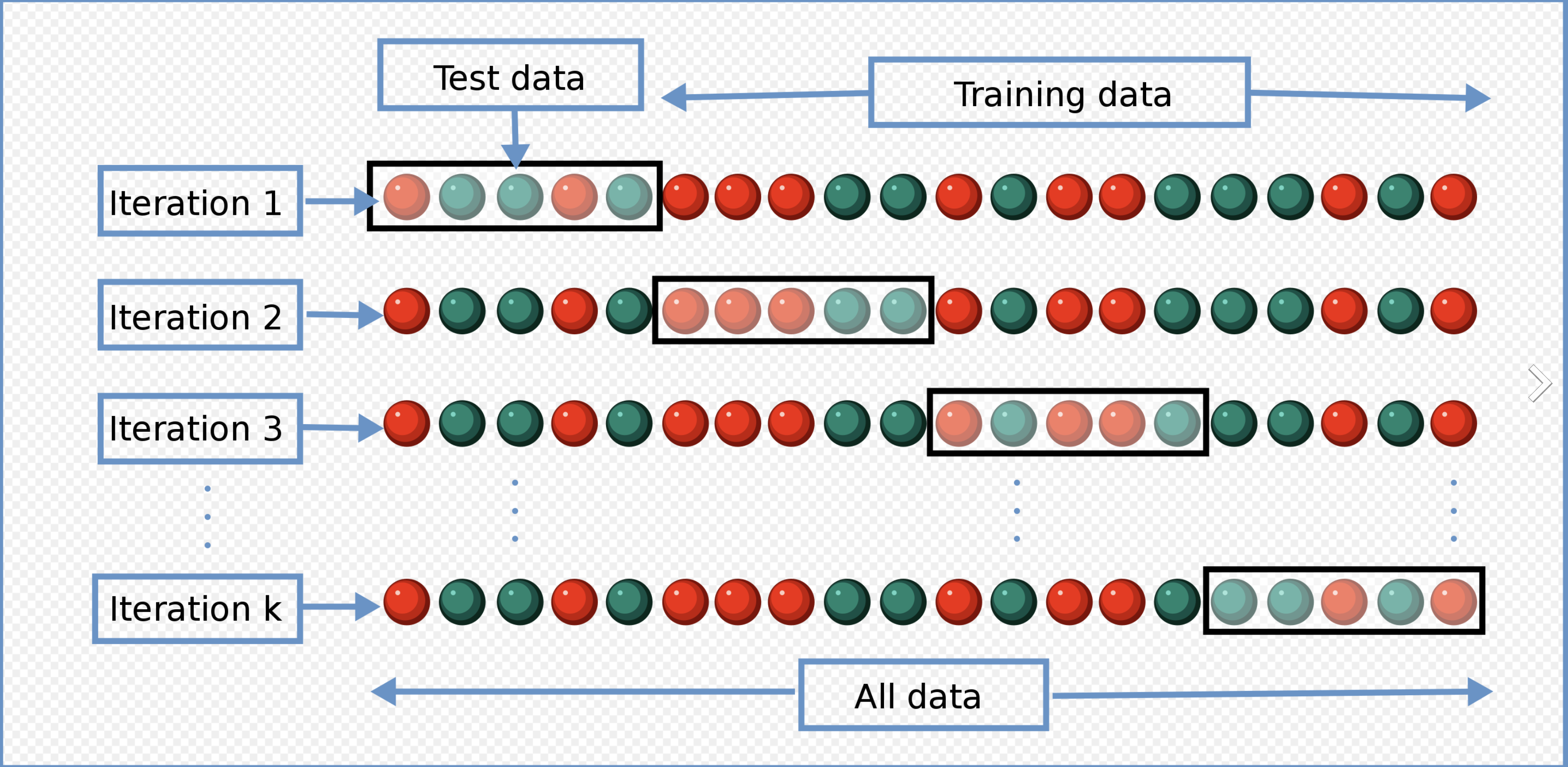
Cross-validation (Source: Wikimedia Commons contributors (2016))
Review: An Introduction to Statistical Learning (James et al. 2013), Chapter 5.1
A general penalty/regulariser
Regularization term: \mathrm{Err}_W(\bm{w}) = \sum_{j=1}^{M} |w_j|^q = \lVert \bm{w} \rVert^q
The regularised error is \tilde{\mathrm{Err}}(\bm{w}) = \sum_{n=1}^{N} [f(x_n, \bm{w}) - t_n]^2 + \lambda \lVert \bm{w} \rVert^q
q=1: L1 regularisation (lasso)
q=2: L2 regularisation (ridge)
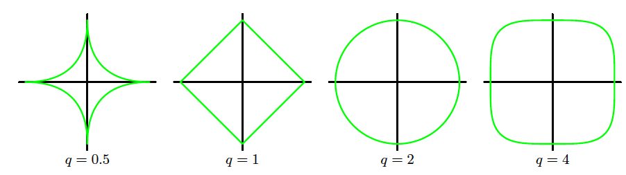
Geometric interpretation of L1 and L2 regularisation (Source: Bishop and Nasrabadi (2006), Figure 3.3)
Geometric Comparison of Ridge and Lasso
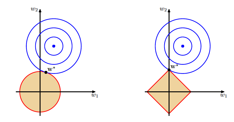
Geometric comparison of ridge and lasso regularisation (Source: Bishop and Nasrabadi (2006), Figure 3.4)
Effect of Regularisation Strength
- M=9
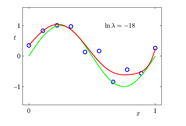
Fitted model (ln λ = -18, weak regularisation) (Source: Bishop and Nasrabadi (2006), Figure 1.7)
Effect of Regularisation Strength (continued)
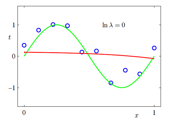
Fitted model (ln λ = 0, strong regularisation) (Source: Bishop and Nasrabadi (2006), Figure 1.7)
RMS Error vs Regularisation
- M=9
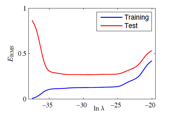
Training and test RMS error versus \ln \lambda (Source: Bishop and Nasrabadi (2006), Figure 1.8)
Too Simple: Linear Model Misspecification
Using (x, x^2)
Overfitting
Sometimes, when the feature dimension is large relative to the number of observations, the model can overfit.
Bayesian Interpretation of L_2 (Ridge) Penalty
- The prior distribution g is Gaussian with mean zero and standard deviation that depends on \lambda
- The posterior mode (the most likely value) of \bm{\beta} is the ridge regression solution
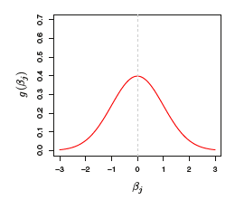
Gaussian prior for ridge regression (Source: An Introduction to Statistical Learning (James et al. 2013), Figure 6.11)
Bayesian Interpretation of L_1 (Lasso) Penalty
- The prior distribution g is a double-exponential (Laplace) distribution with mean zero and scale parameter that depends on \lambda
- The posterior mode of \bm{\beta} is the lasso solution
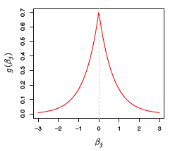
Laplace prior for lasso regression (Source: An Introduction to Statistical Learning (James et al. 2013), Figure 6.11)
Geometry of the Elastic Net
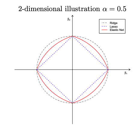
Geometry of ridge, lasso, and elastic net penalties (Source: Zou and Hastie (2004))
The elastic net penalty J(\bm{\beta}) = \alpha \lVert \bm{\beta} \rVert^2 + (1 - \alpha)\lVert \bm{\beta} \rVert_1 where \alpha = \frac{\lambda_2}{\lambda_2 + \lambda_1} - Singularities at the vertexes (necessary for sparsity) - Strict convex edges; the strength of convexity varies with \alpha (grouping effect)
Feature Selection Methods
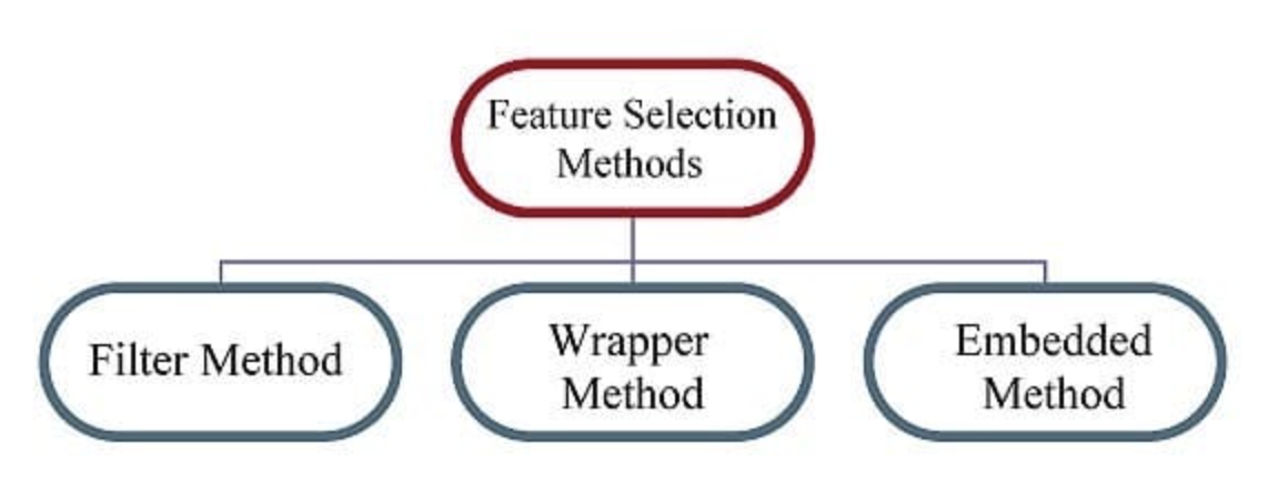
Overview of feature selection methods (Source: Analytics Vidhya (2016), adapted from online sources)
Filter Methods

Filter methods (Source: Analytics Vidhya (2016))
- Used as a data preprocessing step
- Features are selected based on statistical measures of their relationship with the target (response) variable
- Filter methods do not address multicolinearity.
| Feature\Response | Continuous | Categorical |
|---|---|---|
| Continuous | Pearson’s Correlation | LDA |
| Categorical | ANOVA | Chi-square test |
Wrapper Methods

Wrapper methods (Source: Analytics Vidhya (2016))
- Identify subsets of features by training and evaluating a model
- This is a search problem and can be computationally expensive.
Embedded Methods

Embedded methods (Source: Analytics Vidhya (2016))
- Feature selection is built into the model training process
- Example: lasso regression
References
![]()