Actuarial Data Science - Open Learning Resource
Tree-based methods and random forests are powerful yet relatively interpretable approaches for modelling complex, non-linear relationships. In this lecture, we build from single trees to ensembles and focus on practical questions an actuary cares about: how to tune models, how to assess performance, and when these methods are preferable to simpler models.
Understand the motivations behind ensemble learning methods, including bagging and random forests
Construct Classification and Regression Tree (CART).
Perform predictive modelling using random forests, including model fitting, hyperparameter selection, and model assessment
Compare random forests with other modelling techniques
Classifying the iris data using CART (Source: Flower images are from Wikipedia)
Hitters dataset: predict a baseball player’s log salary based on Years and Hits

Let R_m denote a node. The RSS of the response variable in R_m is RSS_m = \sum_{i \in R_m} (y_i - \hat{y}_{R_m})^2 where \hat{y}_{R_m} is the mean of the response variable in R_m.
Let \hat{p}_{mk}=\dfrac{1}{N_m}\sum_{x_i \in R_m}I(y_i = k) represent the proportion of training observations in the mth region/node that belong to the kth class.
Classification error: E = 1 - \max_k(\hat{p}_{mk})
Gini index: G = \sum_{k=1}^{K}\hat{p}_{mk}(1 - \hat{p}_{mk})
Cross-entropy: D = -\sum_{k=1}^{K}\hat{p}_{mk}\ln(\hat{p}_{mk})
The lower these measures, the more homogeneous the response values in that group.
Comparison of impurity measures for two-class classification (Source: The Elements of Statistical Learning (Hastie et al. 2009), Figure 9.3).
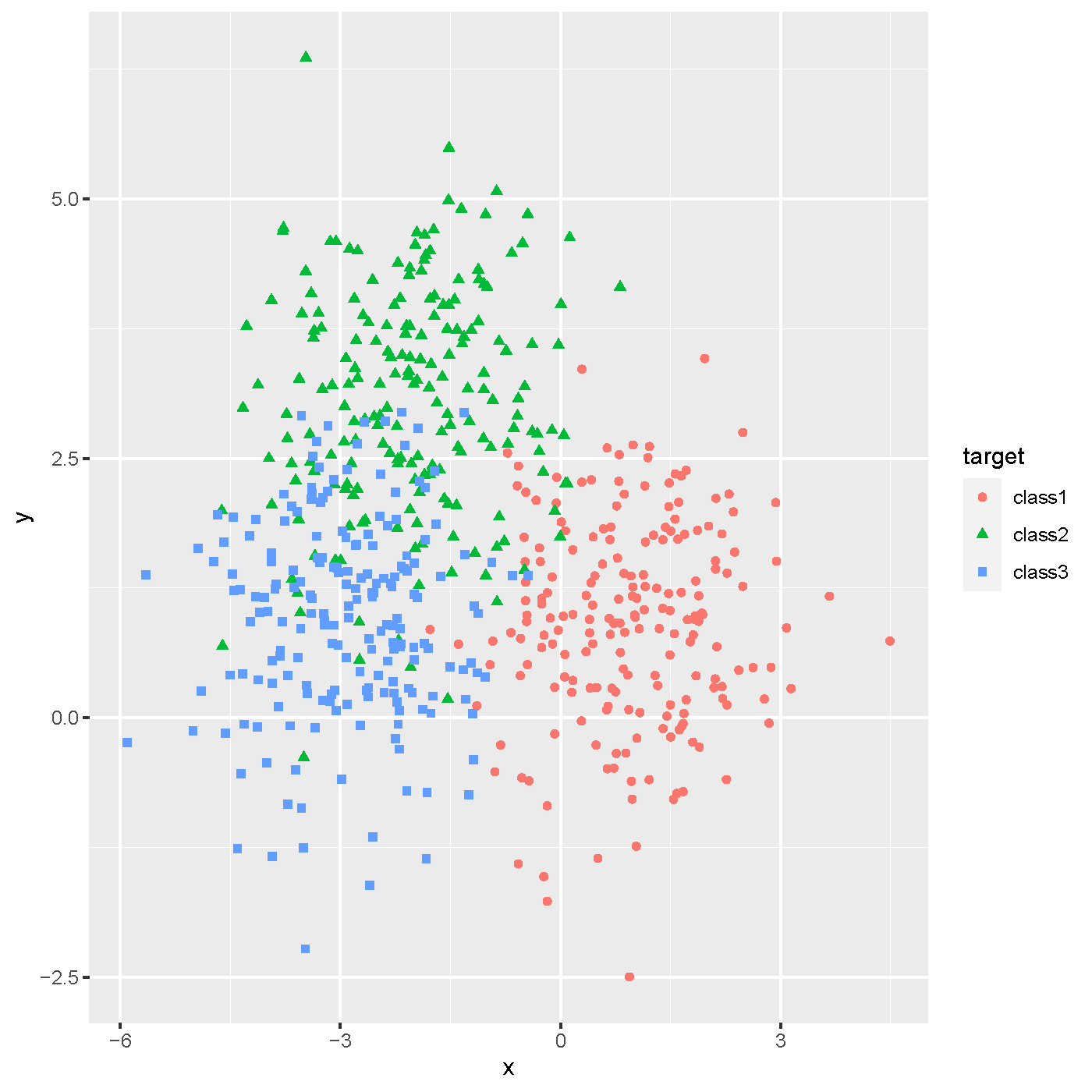
Simulated data with three classes.
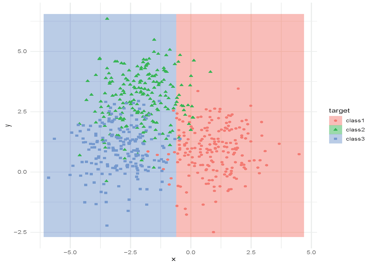
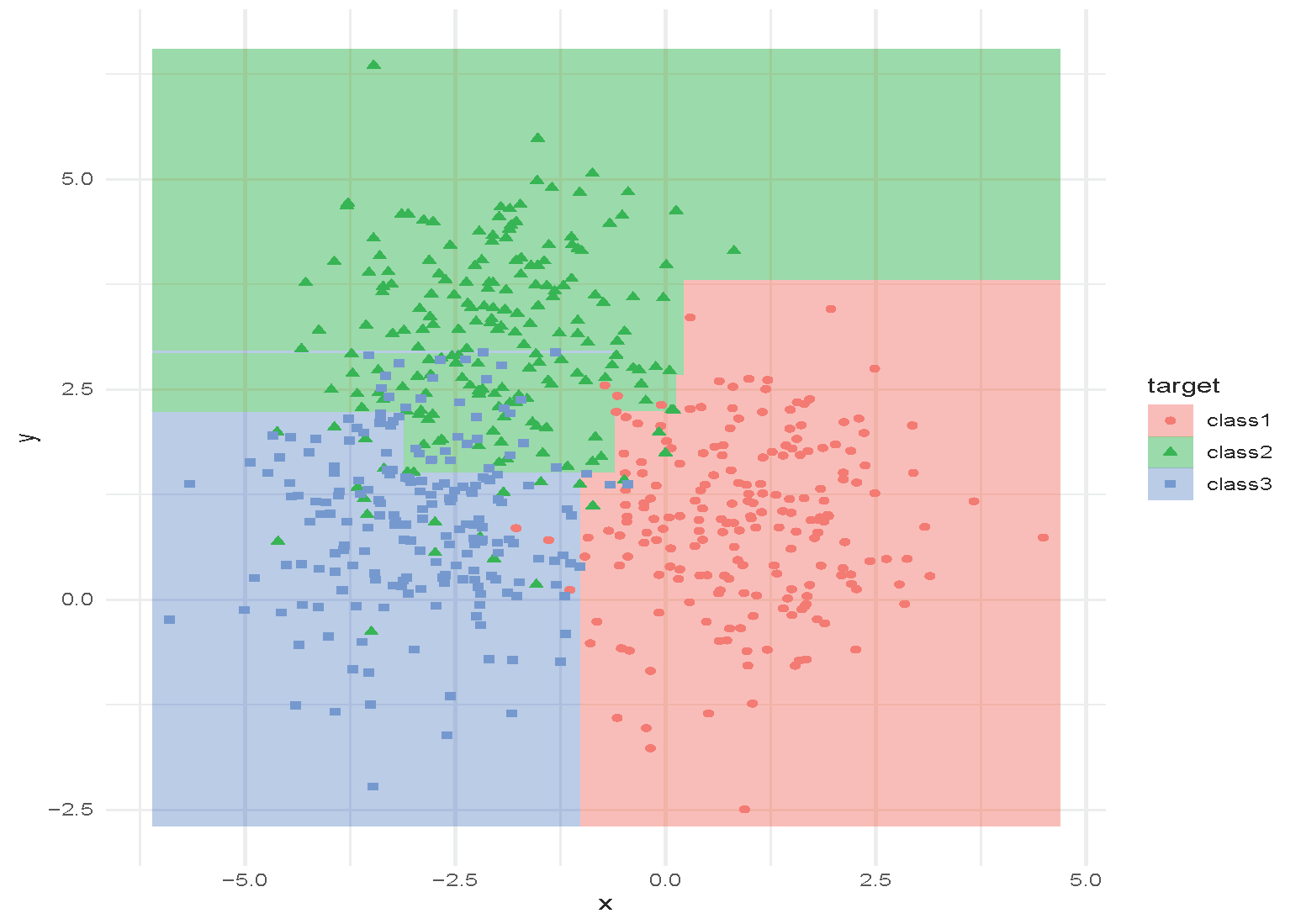
Tree with depth = 1.
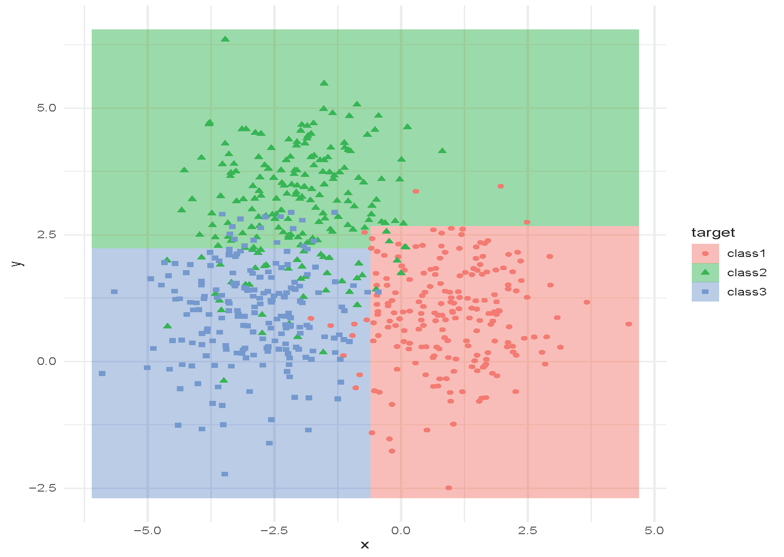
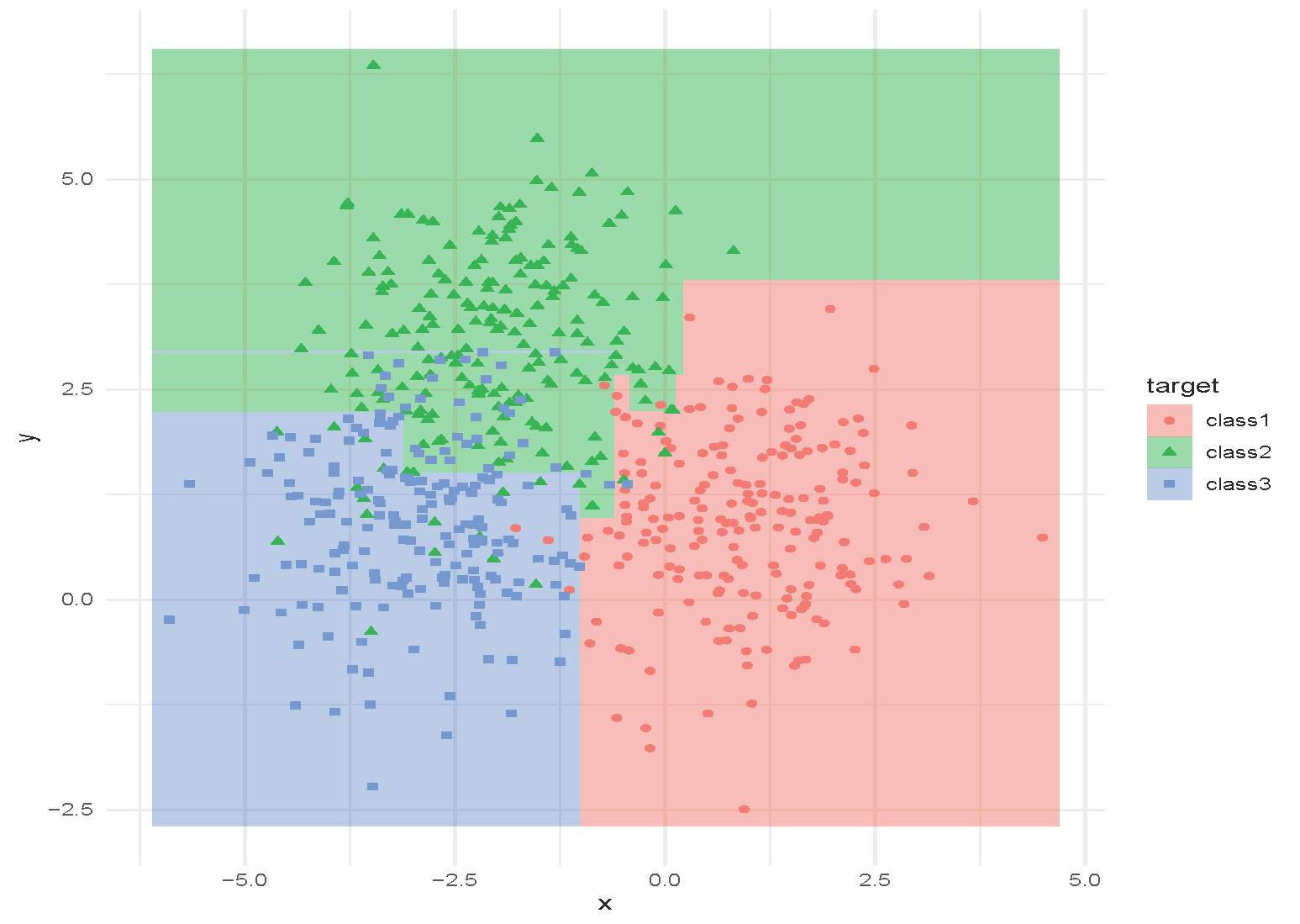
Tree with depth = 2.
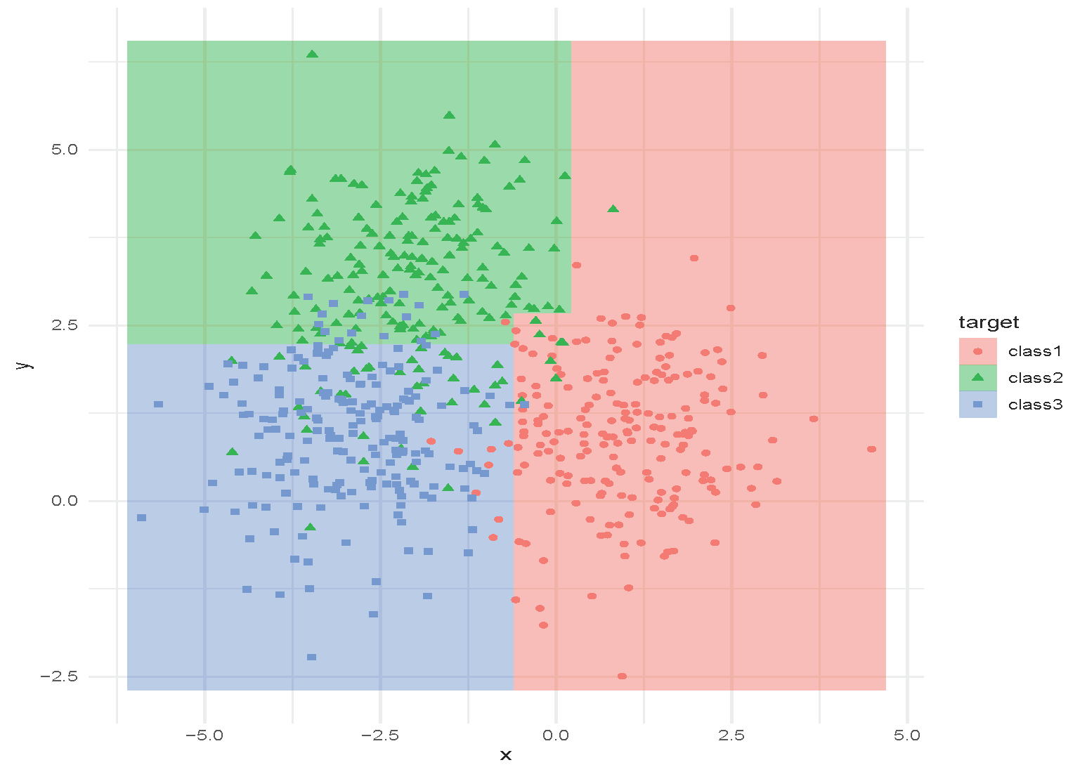
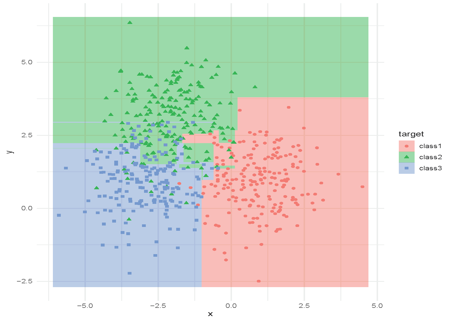
Tree with depth = 3.
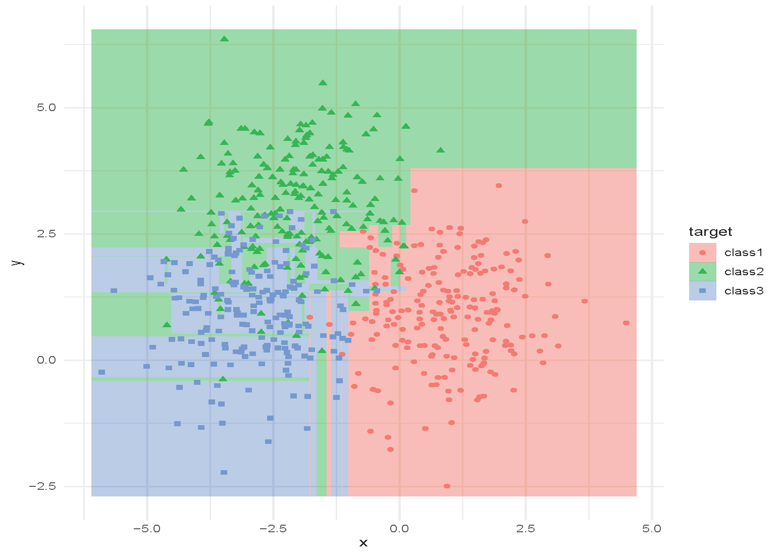
Tree with depth = 4.
Tree with depth = 5.
Tree with depth = 6.
Tree with depth = 15.
[Add a example picture of Regression Tree here]
| GLM | CART | |
|---|---|---|
| Model | Y \mid X \sim \text{Exponential family}; g(\mu)=X^T\beta | A tree with binary splits |
| Continuous predictors | \Phi_j(x)\beta, where \Phi is the linear basis function of x | Tree splits based on the value of a continuous predictor |
| Categorical predictors | binarisation or selecting a baseline level | Tree splits according to categorical levels, e.g. X = a, b, c; left split: X = a, b, right split: X = c |
| Interactions | Need to be manually included in the model | Automatically incorporated via mixed splits |
| Collinearity | A major issue: inflates variance of coefficient estimates and predictions, leads to non-unique estimates and reduced interpretability | Less of an issue, but can affect variable importance measures |
Can be applied to both regression and classification problems; applicable to CART and other statistical machine learning models.
The first method to improve CART using ensemble methods is to train a number of CARTs, each trained on a bootstrapped dataset. The average of their outputs is then used as the final prediction.
A general-purpose procedure to reduce the variance of a statistical learning method
This often performs better than a single CART.
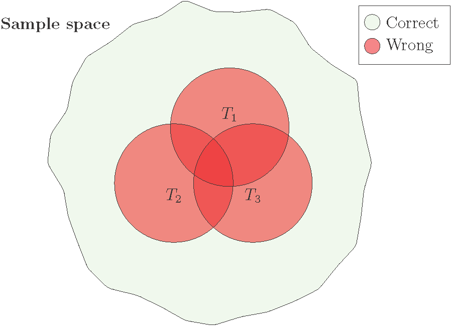
Illustration of bagging with three CART models: overall performance improves when the error regions overlap less.
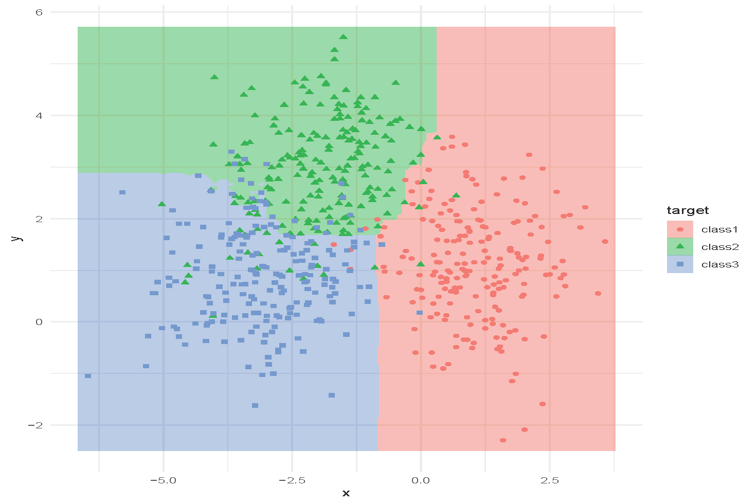
Random forest with n_{\text{trees}} = 1000 and minimum node size = 20.
Hyperparameters:
These can be selected using cross-validation. Random forests are often not very sensitive to these parameters (a strong off-the-shelf predictor).
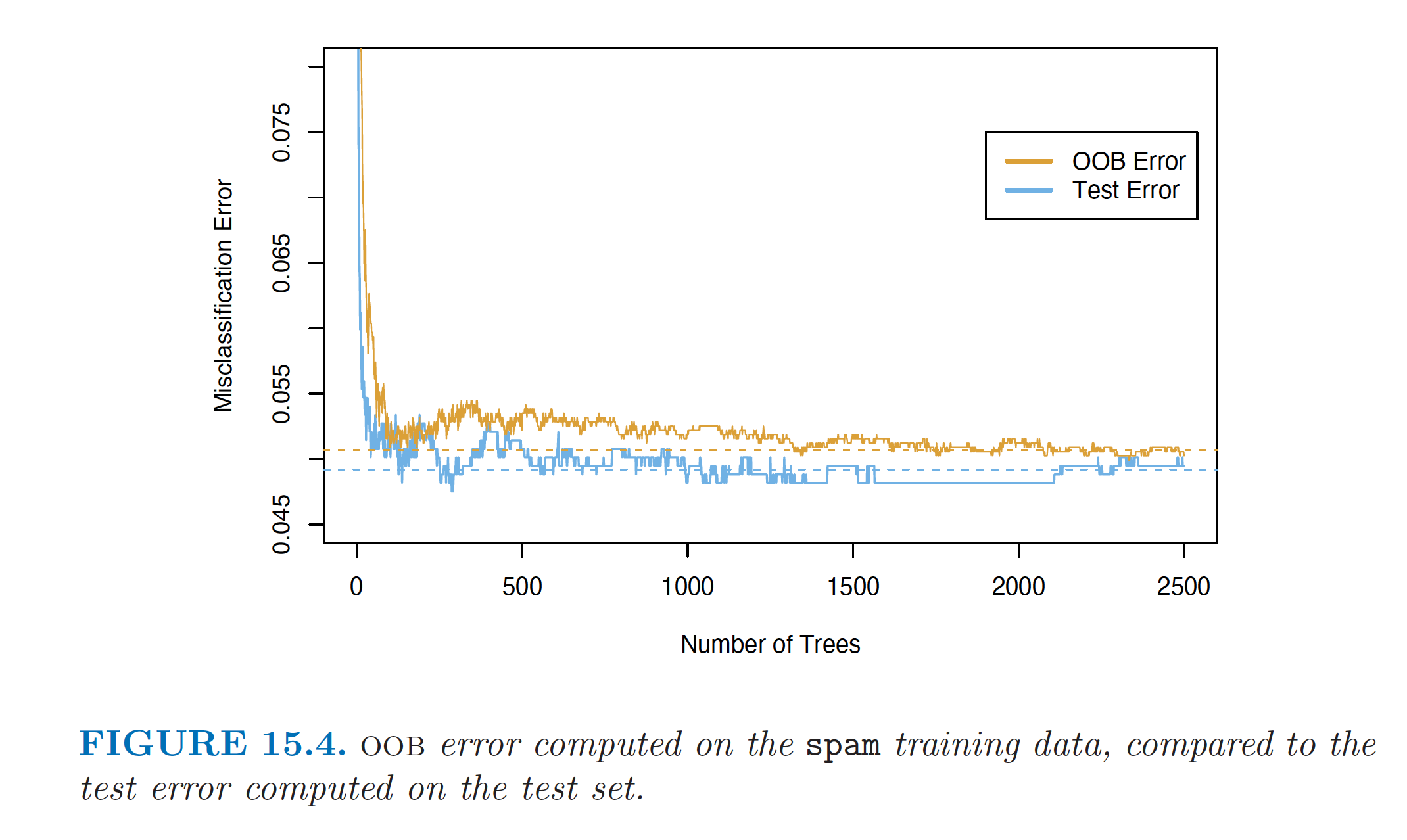
OOB error vs. test error (Source: The Elements of Statistical Learning (Hastie et al. 2009), Figure 15.4).
A similar feature importance measure can be used for bagging by considering the average reduction in RSS or Gini index over all trees for each variable.
The OOB samples can also be used to construct an alternative variable importance measure that reflects the predictive strength of each variable.
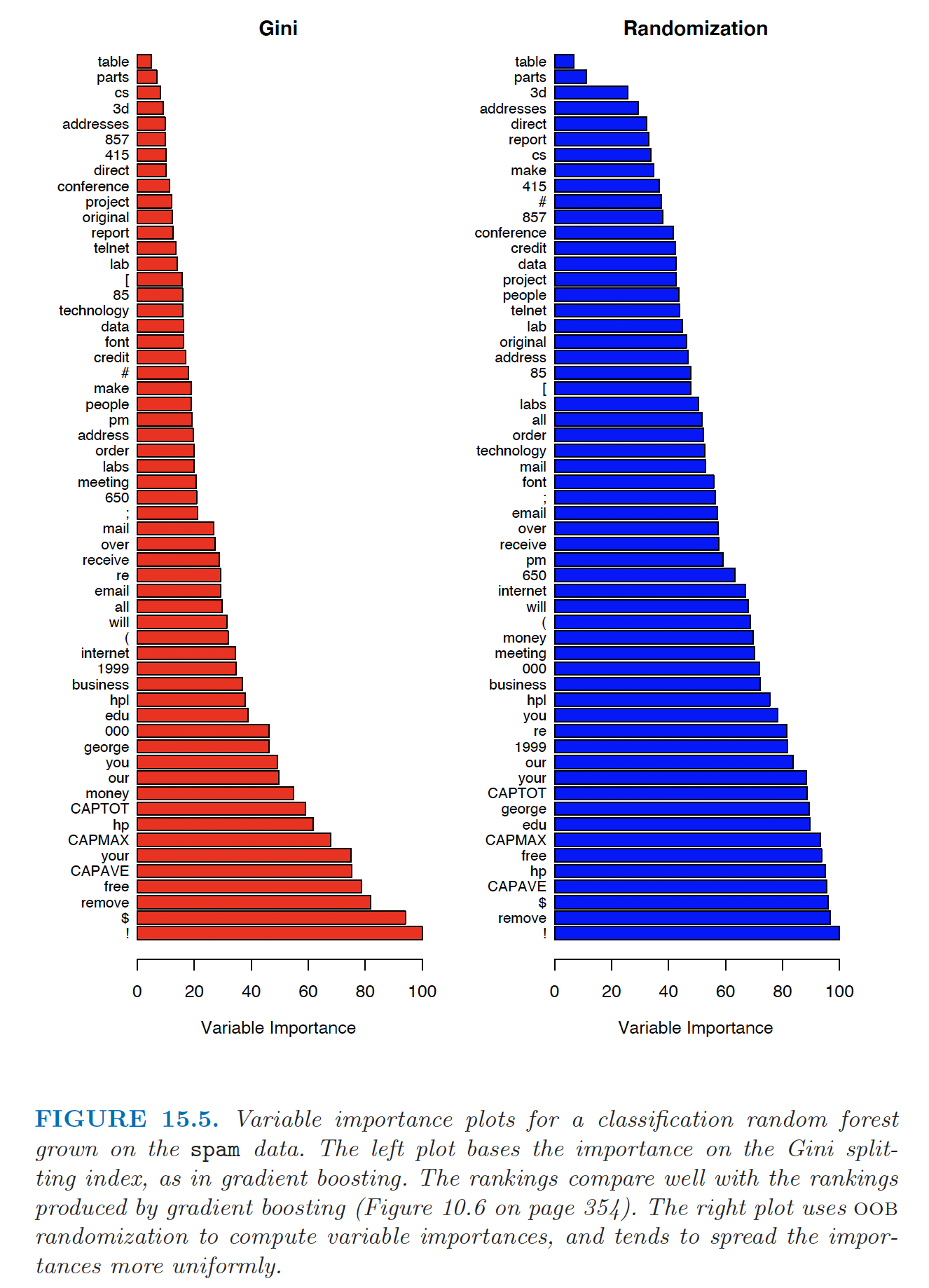
Feature importance based on Gini index (left) and permutation (right) (Source: The Elements of Statistical Learning (Hastie et al. 2009), Figure 15.5).
library(trees)libary(rpart)library(randomForest)library(caret)Review: An Introduction to Statistical Learning (James et al. 2013), Chapter 8.3 (Lab)
Mortality modelling is an important topic in life insurance, used in the management of longevity/mortality risk and in the actuarial pricing of mortality-linked securities and joint-life products. Traditionally, regression-based models (such as GLMs) and extrapolative fitting techniques (e.g., ARIMA) have been used to model mortality.
In Deprez, Shevchenko, and Wüthrich (2017), regression trees are used both to illustrate how mortality modeling can be improved by accounting for feature components of an individual and to estimate conditional probabilities related to the cause of mortality. The analysis is based on Swiss mortality data from the Human Mortality Database.
Kopinsky (2017) uses tree-based models to fit and predict maternity recovery rates and mortality rates. The data for this study comprise between 500,000 and 3,000,000 records and were extracted from a selected Group Long-Term Disability Database (more detail available in the paper).
Traditionally, health actuaries use simple claims data to set premium and reserves. Nowadays, they have access to large volumes of clients’ personal , claims, and medical information. Actuaries increasingly use advanced visualisation techniques and other machine-learning methods.
Diana et al. (2019) use machine-learning methods such as GLM, regression trees, random forests, and Bayesian analysis to model insurance claims.
Boodhun and Jayabalan (2018) use machine-learning algorithms, including random forests, to predict applicants’ risk levels. The dataset is from Prudential Life Insurance and contains nearly 60,000 applications with 128 attributes characterising the applicants.
Claims are typically modeled using GLMs. Other machine-learning techniques, such as tree-based methods, copula regression, and kernel regression, are now also used.
