Lab: Markdown and Reproducible Reports

Actuarial Data Science - Open Learning Resource

Author

Fei Huang, UNSW Sydney

Learning Objectives

Learn how to use Markdown and reproducible reporting tools to write academic reports
Understand the differences between R Markdown, Quarto, and other markdown-based reporting frameworks
Practice creating reproducible documents with embedded code in both R and Python

Markdown and Reproducible Reports Introduction

This is a Markdown document that can be used to create HTML, PDF, and MS Word documents with embedded code. Markdown is a simple formatting syntax that is widely used for creating reproducible reports. This lab introduces various markdown-based reporting frameworks, including R Markdown, Quarto, and Jupyter notebooks.

Why Use Markdown for Reproducible Reports?

There are many advantages to using Markdown-based reporting in your work:

Reproducibility: Code and outputs are directly embedded in the document, ensuring results can be reproduced
Automation: When data or code changes, all outputs (figures, tables, numbers) are automatically updated
Version Control: Markdown files work well with Git and other version control systems
Multiple Output Formats: Create HTML, PDF, Word, and presentation slides from the same source
Collaboration: Easy to share and collaborate on documents with embedded code
Cross-Platform: Works on Windows, Mac, and Linux

Available Frameworks

R Markdown

Primary Language: R
Package: rmarkdown
Strengths: Excellent R integration, mature ecosystem, extensive customisation
Best For: R-focused projects, statistical analysis, and academic publishing

Quarto

Primary Languages: R, Python, Julia, Observable JavaScript
Package: quarto
Strengths: Multi-language support, modern features, and excellent documentation
Best For: Multi-language projects, modern workflows, and cross-language collaboration

Jupyter Notebooks

Primary Languages: Python, R, Julia, and many others
Format: .ipynb files
Strengths: Interactive computing, rich output, and extensive language support
Best For: Data science, machine learning, and interactive analysis

Other Options

Bookdown: An extension of R Markdown for books and long documents
Distill: An R Markdown extension for scientific and technical writing
Hugo: A static site generator with Markdown support

In this course, we will primarily use Quarto (.qmd).

Installation

For R Markdown

Before installing R Markdown, you need to have R and RStudio installed:

Install R: Go to R Project and choose the correct version for your system
Install RStudio: Go to RStudio and install the appropriate version
Install rmarkdown: Open RStudio and run:

# install.packages("rmarkdown")

For Quarto

Quarto is the newest and most versatile option:

Install Quarto: Go to Quarto and download the installer
Install R: If using R with Quarto, install R as above
Install Python: If using Python with Quarto, install Python from python.org

For Jupyter Notebooks

Install Python: Download from python.org
Install Jupyter: Open terminal/command prompt and run:
```
pip install jupyter
```
Install R kernel (optional): If you want to use R in Jupyter:
```
install.packages("IRkernel")
IRkernel::installspec()
```
Note: For PDF output, you will need a LaTeX distribution. We recommend TinyTeX:

```{r}
#| echo: true

# To install TinyTeX (works with R Markdown and Quarto)
tinytex::install_tinytex()

# To uninstall TinyTeX
tinytex::uninstall_tinytex()
```

Creating Your First Document

R Markdown

In RStudio, click “File” → “New File” → “R Markdown”:

Quarto

In RStudio, click “File” → “New File” → “Quarto Document”, or create a new .qmd file manually.

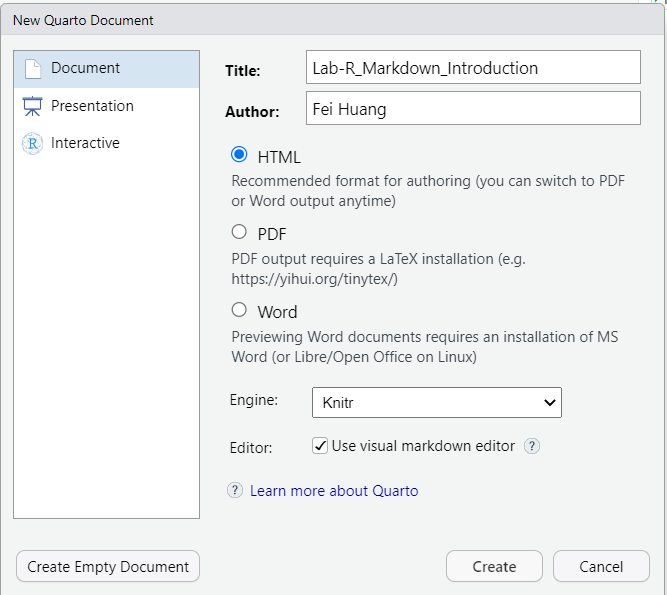
Add the following YAML header:

---
title: "My Report"
format: html
---

Jupyter

Open a terminal/command prompt and run:

jupyter notebook

Note

From this point onwards, we will primarily focus on Quarto (.qmd) for reproducible reporting.

Document Structure

YAML Header

The YAML header controls document metadata and output format:

---
title: "My Amazing Report"
author: "Your Name"
date: today
format:
  html: default
  pdf: default
bibliography: references.bib
---

Markdown Content

Markdown provides simple formatting:

Bold and italic text
Lists and numbered lists
Headers with #, ##, ###
Links: GitHub
Images: ![Caption](image.png)

Code Chunks

Embed executable code in your document:

R in Quarto:

```{r}
# Your R code here
```

Python in Quarto:

```{python}
# Your Python code here
```

Code Chunk Options

Control how code chunks behave (specified using #| in Quarto):

echo: false — Hide code, show results
results: "hide" — Show code, hide results
include: false — Hide both code and results
warning: false — Suppress warnings
message: false — Suppress messages
fig-width: 6, fig-height: 4 — Control figure size

Example with Options

set.seed(123)
x <- rnorm(100)
y <- 2 * x + rnorm(100)
cor(x, y)

Note

The result is hidden due to results: "hide", which looks like the following:

```{r}
#| label: simulate-data
#| echo: true
#| results: "hide"
#| warning: false

set.seed(123)
x <- rnorm(100)
y <- 2 * x + rnorm(100)
cor(x, y)
```

import numpy as np

np.random.seed(123)
x = np.random.normal(0, 1, 100)
y = 2*x + np.random.normal(0, 1, 100)
print(f"Correlation: {np.corrcoef(x, y)[0,1]:.3f}")

Correlation: 0.918

Python Setup

If you encounter errors such as “No module named …”, you may need to install the required Python packages.

You can install them using:

pip install package_name

For example:

pip install numpy matplotlib seaborn

Creating Visualisations

R Example

plot(x, y, main="Scatter Plot", xlab="X", ylab="Y")
abline(lm(y ~ x), col="red")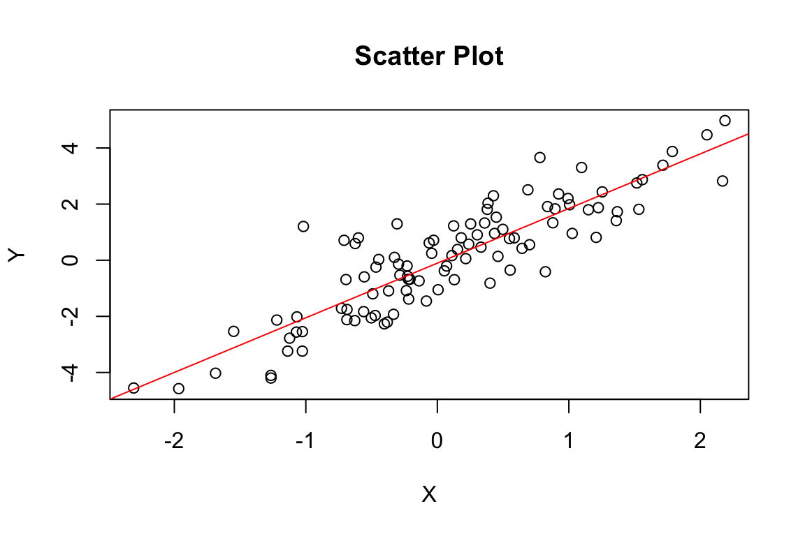

Python Example

# Requires matplotlib in the Python used by R (reticulate). Set eval: true locally after py_install("matplotlib") if needed.

import matplotlib.pyplot as plt

plt.figure(figsize=(6, 4))
plt.scatter(x, y, alpha=0.6)
plt.plot(x, 2*x, color="red", linestyle='--')
plt.xlabel('X')
plt.ylabel('Y')
plt.title('Scatter Plot')
plt.show()

Inline Code

Embed code results directly in your text:

R in Quarto:

Markdown Syntax: There are {r} length(x) data points
- Output: There are 100 data points
Markdown Syntax: The correlation is {r} round(cor(x,y), 3)
- Output: The correlation is 0.879

Python in Quarto:

Markdown Syntax: There are {python} len(x) data points
- Output: There are {python} len(x) data points
Markdown Syntax: The correlation is {python} f"{np.corrcoef(x, y)[0,1]:.3f}"
- Output: The correlation is {python} f"{np.corrcoef(x, y)[0,1]:.3f}"

Note: Inline Python

Inline Python expressions require a Python engine to be enabled in Quarto. In some environments, the Python results above may not display correctly.

To enable inline Python in Quarto, the following conditions are typically required:

Enable the Python engine
Add the following to your YAML header:
```
jupyter: python3
```
However, this changes the execution engine of the document to Python (Jupyter). As a result, R code chunks may no longer run as expected without additional configuration. Therefore, inline Python is not recommended when mixing R and Python in the same document.
Quarto version requirement
Inline Python requires Quarto v1.4 or later. You can check your installed version by running the following in the RStudio Console:
```
system("quarto --version")
```
We recommend installing a version slightly above v1.4. Using the latest version is not necessary and may cause issues when rendering .qmd files.
Updating Quarto
Even after installing a newer version of Quarto, RStudio may continue to use its bundled version unless the system PATH is updated. You may need to install Quarto into the RStudio Quarto directory, overwriting the bundled version used by RStudio. For example:
```
C:/Program Files/RStudio/resources/app/bin/quarto
```

Output Formats

Quarto supports multiple output formats from the same .qmd file:

HTML (`html`)

Interactive elements
Responsive design
Easy to share online

PDF (`pdf`)

Professional appearance
Suitable for printing
Requires LaTeX

Word (`docx`)

Easy to edit further
Familiar to many users
Suitable for collaboration

Presentations

RevealJS (format: revealjs) — HTML slides
Beamer (format: beamer) — PDF slides
PowerPoint (format: pptx) — PowerPoint slides

Best Practices

Reproducibility

Avoid hard-coding results in your text
Use inline code for numbers and statistics
Set random seeds for reproducible results
Document your data sources

Organisation

Use meaningful chunk labels
Group related code chunks together
Keep chunks focused on single tasks
Use comments to explain complex code

Version Control

Track your .qmd files in Git
Do not track generated output files
Use .gitignore to exclude temporary files

Task: Create Your First Report

Create a new Quarto document (.qmd)
Add a YAML header with your information
Write a brief introduction about reproducible reporting
Create a code chunk that generates some data
Create a visualisation
Add inline code to report statistics
Render your document to HTML and PDF

Resources

Quarto: Quarto Documentation
Markdown: Markdown Guide
R Markdown (optional reference): R Markdown: The Definitive Guide
Jupyter (optional reference): Jupyter Documentation

Quarto Introduction

Three Components

Quarto documents rely on three main components:

Markdown for formatted text
Code chunks for executable code (R, Python, etc.)
YAML for document metadata and output formats

Markdown for Formatted Text

Markdown is a set of conventions for formatting plain text. You can use Markdown to indicate:

Bold and italic text: Surround italic text with asterisks, like this without realising it. Surround bold text with two asterisks, like this easy to use.

Examples:

Markdown Syntax	Output
`bold text`	bold text
`italic text`	italic text

Lists: Group lines into bullet points that begin with asterisks or hyphens. Leave a blank line before the first bullet.

Examples:

Markdown Syntax	Output
`- Item 1 - Sub-item 1 - Sub-item 2 - Item 2`	Item 1 Sub-item 1 Sub-item 2 Item 2
`1. First item 2. Second item`	First item Second item

Headers (e.g., section titles): Place one or more hashtags at the start of a line to create a header (or sub-header). For example, # Say Hello to Markdown. A single hashtag (#) creates a first-level header, two hashtags (##) create a second-level header, and so on.
Hyperlinks: Create clickable links using [text](url).

Examples:

Markdown Syntax	Output
`[GitHub](https://github.com)`	GitHub
`[Stack Overflow](https://stackoverflow.com)`	Stack Overflow
`[Reddit](https://www.reddit.com)`	Reddit

and much more

The conventions of Markdown are simple and unobtrusive, making Markdown documents easy to read and write.

You can access a quick guide in RStudio via → “Help” → “Markdown Quick Reference”.

For more details, see the Quarto guide on Markdown Basics.

Chunks

Now, you are familiar with Markdown and Quarto. Quarto supports code chunks that allow you to include executable R or Python code directly in your document, making it easy to create reproducible reports.

Code Chunks

You can use CTRL + ALT + I (Windows) or OPTION + COMMAND + I (Mac) to insert a new code chunk.

It is good practice to assign a label to each chunk using #| label:, for example #| label: simulate-data. Labels are optional but must be unique if used. This helps with debugging and cross-referencing.

Chunk Options

In Quarto, chunk options are specified using #| inside the code block.

echo: false: hide code but show results
results: "hide": show code but hide results
include: false: run code but show neither code nor output
warning: false: suppress warnings
message: false: suppress messages

set.seed(123)
x <- rnorm(100) # 100 random variables from a standard normal distribution
y <- 2 * x + rnorm(100)
cor(x, y)

YAML for Render Parameters

title: “your awesome title”
author: “your name”
date: “today” or specify any date

In Quarto, the format field determines the output format when you render a document.

The format field supports the following values:

html: creates HTML output (default)
pdf: creates PDF output
docx: creates Word output

You can also render your document as a slideshow:

revealjs: creates an HTML slideshow
beamer: creates a PDF slideshow
pptx: creates a PowerPoint presentation

Unlike R Markdown, Quarto provides built-in support for cross-referencing, so no additional output format (e.g., bookdown) is required.

Below are examples of format options (each can be used in a complete YAML header).

Examples of Format Options

Table of Contents (TOC)

title: "My Report"
format: 
  html:
    toc: true
    toc-depth: 3

toc: true: enables the table of contents
toc-depth: controls how many header levels are included

Section Numbering

title: "My Report"
format:
  pdf:
    number-sections: true

number-sections: true: adds numbering to section headers

Figure Caption Placement

title: "My Report"
format:
  html:
    fig-cap-location: bottom

fig-cap-location: controls where figure captions appear (top, bottom, or margin)

Code Folding (HTML only)

title: "My Report"
format:
  html:
    code-fold: true

true: folds all code by default (click to expand)
false: shows all code (default)
show: enables folding but keeps code expanded initially

Code folding is only available in HTML output. It does not apply to PDF or Word formats.

Some options may not apply to all formats. More options for each format are available at: HTML, PDF and Revealjs.

Rendering

To render your .qmd file into HTML, PDF, or Word output, click the “Render” button in RStudio.

A drop-down menu allows you to select the output format (if multiple formats are specified in the YAML header). You can try rendering to different formats.
A shortcut on Windows is CTRL + SHIFT + K, and on macOS it is SHIFT + COMMAND + K.

When you render the document, Quarto will process your .qmd file and generate the output based on the YAML settings and Markdown content. The output file will be saved in your working directory, and a preview will be displayed in RStudio.

Advanced Features in Quarto

Figures

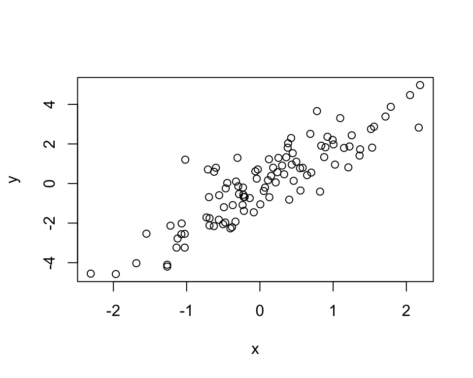
You can control figure appearance using chunk options:

```{r}
#| label: fig-scatterplotfig
#| echo: true
#| fig-width: 5
#| fig-height: 4
#| fig-cap: "Scatterplot"

plot(x,y)
```

Note that:

include: false — hides all code, results, and figures
results: "hide" — hides textual output but keeps figures
fig-show: "hide" — hides figures

Including External Images

You can include an external image using Markdown:

![Caption for the picture.](unsw.jpg).

A more flexible approach is to use a code chunk:

```{r}
#| label: unsw
#| echo: true
#| fig-align: center
#| out-width: "50%"
#| fig-cap: "Welcome to UNSW"

knitr::include_graphics('unsw.jpg')
```

This allows you to control alignment, size, captions, and cross-referencing.

Global Execution and Chunk Options

You may find yourself using similar chunk options throughout a document. Instead of repeating them in every chunk, you can define global defaults at the beginning of the document.

There are two common ways to set global options in Quarto:

Use the YAML header to set document-level options
Use knitr::opts_chunk$set() for R chunks when using the knitr engine

Global Options in the YAML Header

Quarto allows many execution and output options to be set globally in the YAML header. These options apply to the document unless overridden in an individual code chunk.

For example:

---
title: "My Report"
format:
  html:
    code-fold: true
    fig-width: 6
    fig-height: 4
execute:
  echo: true
  warning: false
  message: false

Here: - execute: echo: true shows code by default - execute: warning: false suppresses warnings by default - execute: message: false suppresses messages by default - fig-width and fig-height set the default figure size for the HTML output - code-fold: true enables code folding in HTML output

You can still override these options in a specific chunk. For example:

```{r}
#| echo: false

summary(cars)
```

In this chunk, echo: false overrides the global echo: true.

Note

For more details on available execution and output options, see the Quarto guide on Execution Options.

Global Options for R Chunks Using `knitr`

For R chunks, you can also set global defaults using knitr::opts_chunk$set() in an initial setup chunk:

These options apply to subsequent R chunks unless overridden locally.

For example, you can override the figure height in a specific R chunk:

```{r}
#| label: taller-figure
#| echo: true
#| fig-height: 6
#| fig-cap: "Multiple plots"

par(mfrow=c(2,2))
for(i in 1:4){
  plot(x[(1:25)*i], y[(1:25)*i]) 
}
```

Note

For Quarto documents that mix R and Python, YAML-level options are usually clearer and more consistent. knitr::opts_chunk$set() is mainly for R chunks using the knitr engine and should not be relied on to control Python chunks.

Cross-Referencing

Quarto provides built-in support for cross-referencing figures, tables, equations, and sections.

To create a cross-reference, you need to assign a label to an element. A label is a unique identifier that allows the element to be referenced elsewhere in the document.

Each label uses a prefix to indicate the type of element. Common prefixes include:

sec- for sections
fig- for figures
tbl- for tables
eq- for equations

Once a label is defined, you can refer to it in the text, and Quarto will automatically format the reference and assign numbers where appropriate (e.g., “Section 2”, “Figure 1”, etc.).

Naming tips

Labels must be unique within the document
Use kebab-case (e.g., sec-my-section)
Avoid using underscores (_) in labels

Figures and Tables

We can refer to figures and tables using their labels.

For example, the following figure was defined earlier:

Markdown Syntax: @fig-scatterplotfig
Output: see Figure 2

Table example

To create and reference a table:

```{r}
#| label: tbl-mtcars
#| tbl-cap: "First few rows of mtcars dataset"

knitr::kable(head(mtcars))
```

Example:

knitr::kable(head(mtcars))

Table 1: First few rows of mtcars dataset

	mpg	cyl	disp	hp	drat	wt	qsec	vs	am	gear	carb
Mazda RX4	21.0	6	160	110	3.90	2.620	16.46	0	1	4	4
Mazda RX4 Wag	21.0	6	160	110	3.90	2.875	17.02	0	1	4	4
Datsun 710	22.8	4	108	93	3.85	2.320	18.61	1	1	4	1
Hornet 4 Drive	21.4	6	258	110	3.08	3.215	19.44	1	0	3	1
Hornet Sportabout	18.7	8	360	175	3.15	3.440	17.02	0	0	3	2
Valiant	18.1	6	225	105	2.76	3.460	20.22	1	0	3	1

Markdown Syntax: @tbl-mtcars
Output: see Table 1

Equations

You can write equations using LaTeX syntax:

$$
\bar{X} = \frac{\sum_{i=1}^n X_i}{n}
$$ {#eq-mean}

Example:

\bar{X} = \frac{\sum_{i=1}^n X_i}{n} \tag{1}

Markdown Syntax: @eq-mean
Output: see Equation 1

Sections

You can assign a label to a section by adding {#label} to the header:

### Sections {#sec-sections}

You can then refer to this section in text:

Markdown Syntax: @sec-sections
Output: see Section 3.3.4

Citations

To include references in a Quarto document:

Create a bibliography file: Create a .bib file in the same directory as your .qmd file (e.g., refWeek1.bib).
Add references to the file: You can obtain BibTeX entries from sources such as Google Scholar. For example:
- Search for a paper (e.g., Handbook of Data Visualization)
- Click Cite → BibTeX
- Copy the entry and paste it into your .bib file
Specify the bibliography in YAML: Add the following to your YAML header:
```
bibliography: refWeek1.bib
```
Cite in text: Use @key to cite a reference, where key is the identifier in the .bib file. For example:
- Markdown Syntax: @chen2007handbook
- Output: Chen, Härdle, and Unwin (2007)
Add a reference section: At the end of your document, include:
```
# References
```
Quarto will automatically generate the reference list.

Comments

You can add comments in your document that will not appear in the final output.

<!-- This text will not be displayed in the output -->

Example (no text will appear below because it is commented out):

You can also use the RStudio menu:
click Code → Comment/Uncomment Lines to quickly comment or uncomment selected lines.

Visual Markdown Editor in RStudio

The visual editor is useful for those who are not yet familiar with Markdown or prefer not to write Markdown syntax manually. In RStudio, you can switch between Source mode and Visual mode for a .qmd document by clicking the “Visual” or “Source” button in the editor toolbar.¹

As an exercise, you can experiment with the following features of the visual editor:

Format: bold, italic, underline, code, super^script, sub_script, etc.
Headers: 1st-level header, 2nd-level header, …, 6th-level header
Hyperlinks
Lists (bulleted or numbered)
Insert: citations, cross-references (figures, tables, equations), footnotes, and comments
And so on

In general, the visual editor makes document editing feel more like working in Word. However, for reproducible documents, it is still important to understand the underlying Markdown and Quarto syntax. Be careful when editing YAML headers, code chunks, and LaTeX equations, as visual editing may occasionally change the underlying source in unexpected ways.

References

Chen, Chun-houh, Wolfgang Karl Härdle, and Antony Unwin. 2007. Handbook of Data Visualization. Springer Science & Business Media.

Footnotes

If you do not see this option, please update RStudio to a recent version.↩︎

Learning Objectives

Markdown and Reproducible Reports Introduction

Why Use Markdown for Reproducible Reports?

Available Frameworks

R Markdown

Quarto

Jupyter Notebooks

Other Options

Installation

For R Markdown

For Quarto

For Jupyter Notebooks

Creating Your First Document

R Markdown

Quarto

Jupyter

Document Structure

YAML Header

Markdown Content

Code Chunks

Code Chunk Options

Example with Options

Creating Visualisations

R Example

Python Example

Inline Code

Output Formats

HTML (html)

PDF (pdf)

Word (docx)

Presentations

Best Practices

Reproducibility

Organisation

Version Control

Task: Create Your First Report

Resources

Quarto Introduction

Three Components

Markdown for Formatted Text

Chunks

Code Chunks

Chunk Options

YAML for Render Parameters

Rendering

Advanced Features in Quarto

Figures

Including External Images

Global Execution and Chunk Options

Global Options in the YAML Header

Global Options for R Chunks Using knitr

Cross-Referencing

Figures and Tables

Table example

Equations

Sections

Citations

Comments

Visual Markdown Editor in RStudio

References

Footnotes

HTML (`html`)

PDF (`pdf`)

Word (`docx`)

Global Options for R Chunks Using `knitr`